Asked by Irina Eriomov on Apr 25, 2024

Verified
In the table below are selected values for the OC curve for the acceptance sampling plan n = 210, c = 6. Upon failed inspection, defective items are replaced. Calculate the AOQ for each data point. (You may assume that the population is much larger than the sample.) Plot the AOQ curve. At approximately what population defective rate is the AOQ at its worst? Explain how this happens. How well does this plan meet the specifications of AQL = 0.015, α = 0.05; LTPD = 0.05, β = 0.10? Discuss.
Population percent defective Probability of acceptance 0.001.000000.010.994080.020.866500.030.556230.040.265160.050.100560.060.032170.070.009050.080.002310.090.000540.100.00012\begin{array} { | c | c | } \hline \text { Population percent defective } & \text { Probability of acceptance } \\\hline 0.00 & 1.00000 \\\hline 0.01 & 0.99408 \\\hline 0.02 & 0.86650 \\\hline 0.03 & 0.55623 \\\hline 0.04 & 0.26516 \\\hline 0.05 & 0.10056 \\\hline 0.06 & 0.03217 \\\hline 0.07 & 0.00905 \\\hline 0.08 & 0.00231 \\\hline 0.09 & 0.00054 \\\hline 0.10 & 0.00012 \\\hline\end{array} Population percent defective 0.000.010.020.030.040.050.060.070.080.090.10 Probability of acceptance 1.000000.994080.866500.556230.265160.100560.032170.009050.002310.000540.00012
OC Curve
Operating Characteristic Curve, a graph that describes how well a statistical test or procedure performs in detecting a true condition.
AOQ Curve
is a graphical representation that shows the relationship between the Average Outgoing Quality (AOQ) and the fraction defective in incoming batches, used in quality control to determine the effectiveness of inspection procedures.
Population Defective Rate
The proportion of items in a specified population that are considered to be defective or unsatisfactory.
- Understand acceptance sampling and its application in quality control.
- Calculate and analyze the Average Outgoing Quality (AOQ) in acceptance sampling.

Verified Answer
EW
Emma WilkersonApr 26, 2024
Final Answer :
The plan meets the α and the β specification fairly well.
Population percent defective Probability of acceptance AOQ0.001.0000.00000.010.9940.00990.0150.9580.0144 At AQL 0.020.8670.0173 maximum 0.030.5580.01670.040.2670.01070.050.1020.0051 At LTPD 0.060.0330.00200.070.0090.00060.080.0020.00020.090.0010.0001\begin{array} { | c | c | c | c | } \hline \begin{array} { c } \text { Population percent } \\\text { defective }\end{array} & \begin{array} { c } \text { Probability of } \\\text { acceptance }\end{array} & \mathrm { AOQ } & \\\hline 0.00 & 1.000 & 0.0000 & \\\hline 0.01 & 0.994 & 0.0099 & \\\hline 0.015 & 0.958 & 0.0144 & \text { At AQL } \\\hline 0.02 & 0.867 & 0.0173 & \text { maximum } \\\hline 0.03 & 0.558 & 0.0167 & \\\hline 0.04 & 0.267 & 0.0107 & \\\hline 0.05 & 0.102 & 0.0051 & \text { At LTPD } \\\hline 0.06 & 0.033 & 0.0020 & \\\hline 0.07 & 0.009 & 0.0006 & \\\hline 0.08 & 0.002 & 0.0002 & \\\hline 0.09 & 0.001 & 0.0001 & \\\hline\end{array} Population percent defective 0.000.010.0150.020.030.040.050.060.070.080.09 Probability of acceptance 1.0000.9940.9580.8670.5580.2670.1020.0330.0090.0020.001AOQ0.00000.00990.01440.01730.01670.01070.00510.00200.00060.00020.0001 At AQL maximum At LTPD 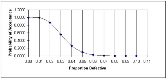
Population percent defective Probability of acceptance AOQ0.001.0000.00000.010.9940.00990.0150.9580.0144 At AQL 0.020.8670.0173 maximum 0.030.5580.01670.040.2670.01070.050.1020.0051 At LTPD 0.060.0330.00200.070.0090.00060.080.0020.00020.090.0010.0001\begin{array} { | c | c | c | c | } \hline \begin{array} { c } \text { Population percent } \\\text { defective }\end{array} & \begin{array} { c } \text { Probability of } \\\text { acceptance }\end{array} & \mathrm { AOQ } & \\\hline 0.00 & 1.000 & 0.0000 & \\\hline 0.01 & 0.994 & 0.0099 & \\\hline 0.015 & 0.958 & 0.0144 & \text { At AQL } \\\hline 0.02 & 0.867 & 0.0173 & \text { maximum } \\\hline 0.03 & 0.558 & 0.0167 & \\\hline 0.04 & 0.267 & 0.0107 & \\\hline 0.05 & 0.102 & 0.0051 & \text { At LTPD } \\\hline 0.06 & 0.033 & 0.0020 & \\\hline 0.07 & 0.009 & 0.0006 & \\\hline 0.08 & 0.002 & 0.0002 & \\\hline 0.09 & 0.001 & 0.0001 & \\\hline\end{array} Population percent defective 0.000.010.0150.020.030.040.050.060.070.080.09 Probability of acceptance 1.0000.9940.9580.8670.5580.2670.1020.0330.0090.0020.001AOQ0.00000.00990.01440.01730.01670.01070.00510.00200.00060.00020.0001 At AQL maximum At LTPD

Learning Objectives
- Understand acceptance sampling and its application in quality control.
- Calculate and analyze the Average Outgoing Quality (AOQ) in acceptance sampling.