EW
Emma Wilkerson
Answers (8)
EW
Answered
U.S. prices rose at an average annual rate of about 3.6 percent over the last 80 years.
On Jul 29, 2024
True
EW
Answered
A graphic design studio is considering three new computers. The first model, A, costs $5000. Model B and C cost $3000 and $1000 respectively. If each customer provides $50 of revenue and variable costs are $20/customer, find the number of customers required for each model to break even.
On Jul 25, 2024
A: BEP = 5000/(50 - 20) = 166.6 customers
B: BEP = 3000/(50 - 20) = 100 customers
C: BEP = 1000/(50 - 20) = 33.3 customers
B: BEP = 3000/(50 - 20) = 100 customers
C: BEP = 1000/(50 - 20) = 33.3 customers
EW
Answered
In profit centers
A) Managers are easy to evaluate because there is a simple metric of how well they performed
B) Managers typically do not have the information to run their division efficiently
C) Managers' decisions rarely affect other divisions
D) Managers typically do not have the incentives to run their division efficiently
On Jun 28, 2024
A
EW
Answered
To maximize total surplus with a monopoly firm, a benevolent social planner would choose the level of output where
A) MR = MC.
B) MR intersects the demand curve.
C) MC intersects the demand curve.
D) MR exceeds MC by the greatest amount.
A) MR = MC.
B) MR intersects the demand curve.
C) MC intersects the demand curve.
D) MR exceeds MC by the greatest amount.
On Jun 25, 2024
C
EW
Answered
Creditors' information needs revolve around all of the following decisions, except
A) extending credit
B) maintaining a credit relationship
C) not extending credit
D) investing in credit instruments
A) extending credit
B) maintaining a credit relationship
C) not extending credit
D) investing in credit instruments
On May 29, 2024
D
EW
Answered
What supplier selection criteria are described by attitude, cultural compatibility, training aids, packaging, and repair service?
A) Sustainability
B) Financial considerations
C) Reliability
D) Desirable qualities
A) Sustainability
B) Financial considerations
C) Reliability
D) Desirable qualities
On May 26, 2024
D
EW
Answered
If your firm had $300,000,the going rate of interest on business loans was 12 percent and your firm's expected profit rate was 17 percent,what would you do with this money?
A) Keep it in the bank.
B) Lend it to a competitor.
C) Use it to finance your own expansion.
A) Keep it in the bank.
B) Lend it to a competitor.
C) Use it to finance your own expansion.
On Apr 29, 2024
C
EW
Answered
In the table below are selected values for the OC curve for the acceptance sampling plan n = 210, c = 6. Upon failed inspection, defective items are replaced. Calculate the AOQ for each data point. (You may assume that the population is much larger than the sample.) Plot the AOQ curve. At approximately what population defective rate is the AOQ at its worst? Explain how this happens. How well does this plan meet the specifications of AQL = 0.015, α = 0.05; LTPD = 0.05, β = 0.10? Discuss.
Population percent defective Probability of acceptance 0.001.000000.010.994080.020.866500.030.556230.040.265160.050.100560.060.032170.070.009050.080.002310.090.000540.100.00012\begin{array} { | c | c | } \hline \text { Population percent defective } & \text { Probability of acceptance } \\\hline 0.00 & 1.00000 \\\hline 0.01 & 0.99408 \\\hline 0.02 & 0.86650 \\\hline 0.03 & 0.55623 \\\hline 0.04 & 0.26516 \\\hline 0.05 & 0.10056 \\\hline 0.06 & 0.03217 \\\hline 0.07 & 0.00905 \\\hline 0.08 & 0.00231 \\\hline 0.09 & 0.00054 \\\hline 0.10 & 0.00012 \\\hline\end{array} Population percent defective 0.000.010.020.030.040.050.060.070.080.090.10 Probability of acceptance 1.000000.994080.866500.556230.265160.100560.032170.009050.002310.000540.00012
Population percent defective Probability of acceptance 0.001.000000.010.994080.020.866500.030.556230.040.265160.050.100560.060.032170.070.009050.080.002310.090.000540.100.00012\begin{array} { | c | c | } \hline \text { Population percent defective } & \text { Probability of acceptance } \\\hline 0.00 & 1.00000 \\\hline 0.01 & 0.99408 \\\hline 0.02 & 0.86650 \\\hline 0.03 & 0.55623 \\\hline 0.04 & 0.26516 \\\hline 0.05 & 0.10056 \\\hline 0.06 & 0.03217 \\\hline 0.07 & 0.00905 \\\hline 0.08 & 0.00231 \\\hline 0.09 & 0.00054 \\\hline 0.10 & 0.00012 \\\hline\end{array} Population percent defective 0.000.010.020.030.040.050.060.070.080.090.10 Probability of acceptance 1.000000.994080.866500.556230.265160.100560.032170.009050.002310.000540.00012
On Apr 26, 2024
The plan meets the α and the β specification fairly well.
Population percent defective Probability of acceptance AOQ0.001.0000.00000.010.9940.00990.0150.9580.0144 At AQL 0.020.8670.0173 maximum 0.030.5580.01670.040.2670.01070.050.1020.0051 At LTPD 0.060.0330.00200.070.0090.00060.080.0020.00020.090.0010.0001\begin{array} { | c | c | c | c | } \hline \begin{array} { c } \text { Population percent } \\\text { defective }\end{array} & \begin{array} { c } \text { Probability of } \\\text { acceptance }\end{array} & \mathrm { AOQ } & \\\hline 0.00 & 1.000 & 0.0000 & \\\hline 0.01 & 0.994 & 0.0099 & \\\hline 0.015 & 0.958 & 0.0144 & \text { At AQL } \\\hline 0.02 & 0.867 & 0.0173 & \text { maximum } \\\hline 0.03 & 0.558 & 0.0167 & \\\hline 0.04 & 0.267 & 0.0107 & \\\hline 0.05 & 0.102 & 0.0051 & \text { At LTPD } \\\hline 0.06 & 0.033 & 0.0020 & \\\hline 0.07 & 0.009 & 0.0006 & \\\hline 0.08 & 0.002 & 0.0002 & \\\hline 0.09 & 0.001 & 0.0001 & \\\hline\end{array} Population percent defective 0.000.010.0150.020.030.040.050.060.070.080.09 Probability of acceptance 1.0000.9940.9580.8670.5580.2670.1020.0330.0090.0020.001AOQ0.00000.00990.01440.01730.01670.01070.00510.00200.00060.00020.0001 At AQL maximum At LTPD 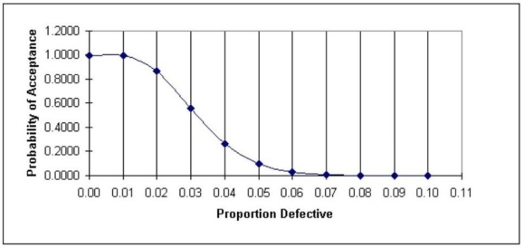
Population percent defective Probability of acceptance AOQ0.001.0000.00000.010.9940.00990.0150.9580.0144 At AQL 0.020.8670.0173 maximum 0.030.5580.01670.040.2670.01070.050.1020.0051 At LTPD 0.060.0330.00200.070.0090.00060.080.0020.00020.090.0010.0001\begin{array} { | c | c | c | c | } \hline \begin{array} { c } \text { Population percent } \\\text { defective }\end{array} & \begin{array} { c } \text { Probability of } \\\text { acceptance }\end{array} & \mathrm { AOQ } & \\\hline 0.00 & 1.000 & 0.0000 & \\\hline 0.01 & 0.994 & 0.0099 & \\\hline 0.015 & 0.958 & 0.0144 & \text { At AQL } \\\hline 0.02 & 0.867 & 0.0173 & \text { maximum } \\\hline 0.03 & 0.558 & 0.0167 & \\\hline 0.04 & 0.267 & 0.0107 & \\\hline 0.05 & 0.102 & 0.0051 & \text { At LTPD } \\\hline 0.06 & 0.033 & 0.0020 & \\\hline 0.07 & 0.009 & 0.0006 & \\\hline 0.08 & 0.002 & 0.0002 & \\\hline 0.09 & 0.001 & 0.0001 & \\\hline\end{array} Population percent defective 0.000.010.0150.020.030.040.050.060.070.080.09 Probability of acceptance 1.0000.9940.9580.8670.5580.2670.1020.0330.0090.0020.001AOQ0.00000.00990.01440.01730.01670.01070.00510.00200.00060.00020.0001 At AQL maximum At LTPD